(Co)variance estimation

ARCH and GARCH

This short exercise illustrates how to perform maximum likelihood estimation using the simple example of ARCH\((p)\) and GARCH(\(p, q\)) models. First, write the code for the basic specification independently. Afterward, the exercises will help you familiarize yourself with well-established packages that provide the same (and much more sophisticated) methods to estimate conditional volatility models.

Exercises:

As a benchmark dataset, download prices and compute daily returns for all stocks that are part of the Dow Jones 30 index (ticker <- "DOW"). The sample period should start on January 1st, 2000. Then, decompose the time series into a predictable part and the residual, \(r_t = E(r_t|\mathcal{F}_{t-1}) + \varepsilon_t\). The most straightforward approach would be to demean the time series by simply subtracting the sample mean, but in principle, more sophisticated methods can be used.
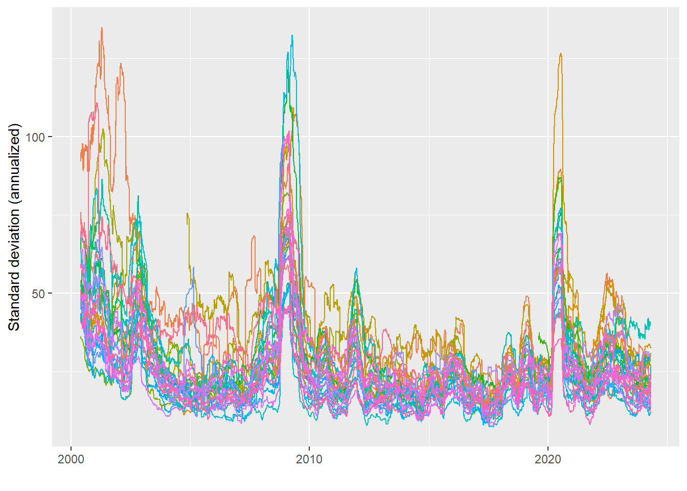
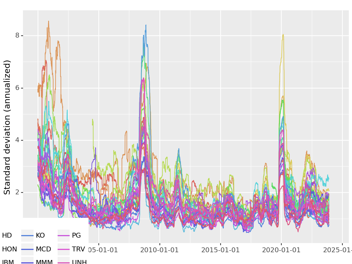
For each of the 30 tickers, illustrate the rolling window standard deviation based on some suitable estimation window length.
Write a small function that computes the maximum likelihood estimator (MLE) of an ARCH(\(p\)) model.
Write a second function implementing MLE estimation for a GARCH(\(p,q\)) model.
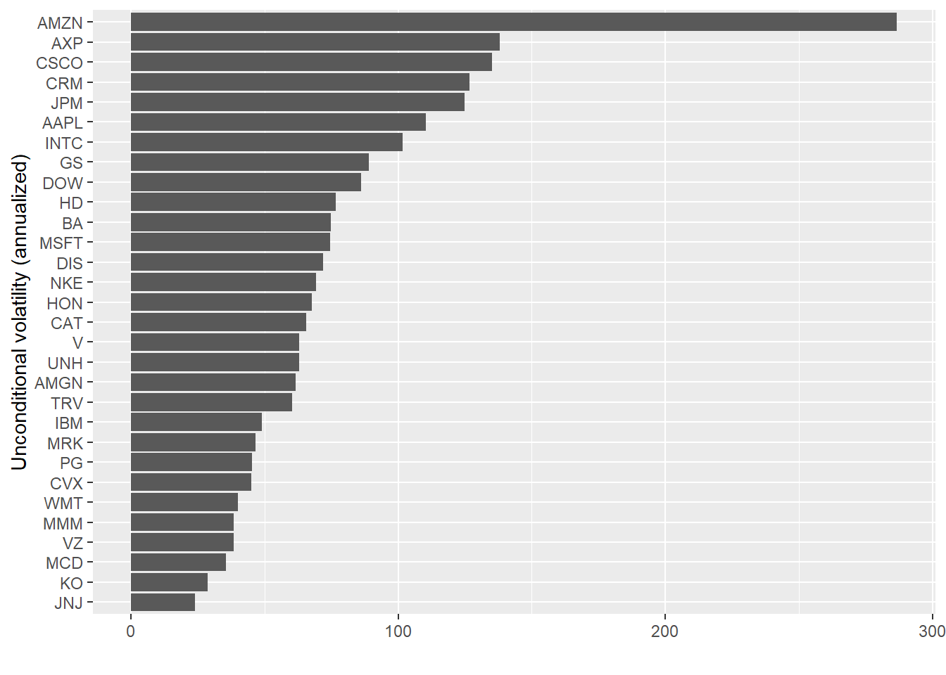
What is the unconditional estimated variance of the ARCH(\(1\)) and the GARCH(\(1, 1\)) model for each ticker?

Compute and illustrate the model-implied Value-at-risk, defined as the lowest return your model expects with a probability of less than 5 %. Formally, the VaR is defined as \(\text{VaR} _{\alpha }(X)= -\inf {\big \{}x\in \mathbb {R} :F_{-X}(x)>\alpha {\big \}}=F_{-X}^{-1}(1-\alpha)\) where \(X\) is the return distribution. Illustrate stock returns that fall below the estimated Value-at-risk. What can you conclude?

Solutions:

R
Python

library(tidyverse)

── Attaching core tidyverse packages ──────────────────────── tidyverse 2.0.0 ──
✔ dplyr     1.1.4     ✔ readr     2.1.4
✔ forcats   1.0.0     ✔ stringr   1.5.1
✔ ggplot2   3.4.4     ✔ tibble    3.2.1
✔ lubridate 1.9.3     ✔ tidyr     1.3.0
✔ purrr     1.0.2     
── Conflicts ────────────────────────────────────────── tidyverse_conflicts() ──
✖ dplyr::filter() masks stats::filter()
✖ dplyr::lag()    masks stats::lag()
ℹ Use the conflicted package (<http://conflicted.r-lib.org/>) to force all conflicts to become errors

library(tidyquant)

Indlæser krævet pakke: PerformanceAnalytics
Indlæser krævet pakke: xts
Indlæser krævet pakke: zoo

Vedhæfter pakke: 'zoo'

De følgende objekter er maskerede fra 'package:base':

    as.Date, as.Date.numeric


######################### Warning from 'xts' package ##########################
#                                                                             #
# The dplyr lag() function breaks how base R's lag() function is supposed to  #
# work, which breaks lag(my_xts). Calls to lag(my_xts) that you type or       #
# source() into this session won't work correctly.                            #
#                                                                             #
# Use stats::lag() to make sure you're not using dplyr::lag(), or you can add #
# conflictRules('dplyr', exclude = 'lag') to your .Rprofile to stop           #
# dplyr from breaking base R's lag() function.                                #
#                                                                             #
# Code in packages is not affected. It's protected by R's namespace mechanism #
# Set `options(xts.warn_dplyr_breaks_lag = FALSE)` to suppress this warning.  #
#                                                                             #
###############################################################################

Vedhæfter pakke: 'xts'

De følgende objekter er maskerede fra 'package:dplyr':

    first, last


Vedhæfter pakke: 'PerformanceAnalytics'

Det følgende objekt er maskeret fra 'package:graphics':

    legend

Indlæser krævet pakke: quantmod
Indlæser krævet pakke: TTR
Registered S3 method overwritten by 'quantmod':
  method            from
  as.zoo.data.frame zoo

import pandas as pd
import numpy as np
from scipy.optimize import minimize
import yfinance as yf
from plotnine import ggplot, aes, geom_line, labs, theme, geom_bar, coord_flip

We download price data of the time series of 30 stocks and compute (adjusted) net returns. Then, I demean the return time series. This step could be replaced by either adjusting return based on some estimated factor model or predictions that stem from the part on Machine Learning.

R
Python

ticker <- tq_index("DOW")

Getting holdings for DOW

index_prices <- tq_get(ticker,
  get = "stock.prices",
  from = "2000-01-01"
)

Warning: There was 1 warning in `dplyr::mutate()`.
ℹ In argument: `data.. = purrr::map(...)`.
Caused by warning:
! x = '-', get = 'stock.prices': Error in getSymbols.yahoo(Symbols = "-", env = <environment>, verbose = FALSE, : Unable to import "-".
HTTP error 404.
 Removing -.

returns <- index_prices |>
  group_by(symbol) |>
  mutate(ret = 100 * (adjusted / lag(adjusted) - 1)) |>
  select(symbol, date, ret) |>
  drop_na(ret) |>
  mutate(ret = ret - mean(ret))


# Define the URL to fetch ticker symbols
url = ("https://www.ssga.com/us/en/institutional/etfs/library-content/"
       "products/fund-data/etfs/us/holdings-daily-us-en-dia.xlsx")

# Fetch ticker symbols from the URL
symbols = (pd.read_excel(url, skiprows=4, nrows=30)
           .get("Ticker")
           .tolist()
          )

# Download price data for the fetched ticker symbols

index_prices = (yf.download(
    tickers=symbols, 
    start="2000-01-01", 
     progress=False
  )
  .melt(ignore_index=False, var_name=["variable", "symbol"])
  .reset_index()
  .pivot(index=["Date", "symbol"], columns="variable", values="value")
  .reset_index()
  .rename(columns={
    "Date": "date", 
    "Open": "open", 
    "High": "high", 
    "Low": "low",
    "Close": "close", 
    "Adj Close": "adjusted", 
    "Volume": "volume"}
  )
)    

returns = (index_prices.groupby('symbol')
           .apply(lambda group: group.assign(ret=100 * (group['adjusted'] / group['adjusted'].shift(1) - 1)))
           .reset_index(drop=True)
           .loc[:, ['symbol', 'date', 'ret']]
           .dropna()
           .assign(ret=lambda df: df['ret'] - df.groupby('symbol')['ret'].transform('mean'))
          )

R
Python

library(slider)

rolling_sd <- returns |> 
  group_by(symbol) |> 
  mutate(rolling_sd = slide_dbl(ret, sd, 
                                .before = 100,
                                .complete = TRUE)) # 100 day estimation window

rolling_sd |>
  drop_na() |> 
  ggplot(aes(x=date, 
             y = sqrt(250) * rolling_sd, 
             color = symbol)) + 
  geom_line() +
  labs(x = "", y = "Standard deviation (annualized)") +
  theme(legend.position = "None")

Similar to the Chapter on beta estimation, I use the slider package for convenient rolling window computations. For detailed documentation, consult (this homepage.)[https://github.com/DavisVaughan/slider]. The option `.complete = TRUE’ ensures that the rolling standard deviations are only computed if sufficient data is available.

def roll_sd(data, window_size):
    """Calculate rolling standard deviation."""
    rolling_sd = data['ret'].rolling(window=window_size).std().shift(-window_size + 1)
    return rolling_sd

# Assuming 'returns' is your DataFrame
window_size = 100  # Specify the window size
rolling_sd = returns.assign(
    rolling_sd=returns.groupby('symbol', dropna=False).apply(roll_sd, window_size=window_size).reset_index(level=0, drop=True)
)

(ggplot(rolling_sd, aes(x='date', y='rolling_sd', color='symbol')) +
 geom_line() +
 labs(x="", y="Standard deviation (annualized)") +
 theme(legend_position="None"))

<Figure Size: (640 x 480)>

C:\Users\ncj140\DOCUME~1\VIRTUA~1\R-RETI~1\lib\site-packages\plotnine\geoms\geom_path.py:98: PlotnineWarning: geom_path: Removed 99 rows containing missing values.

The figure illustrates at least two relevant features: i) Although rather persistent, volatilities change over time, and ii) volatilities tend to co-move. Next, I write a simplified script that performs maximum likelihood estimation of the parameters of an ARCH(\(p\)) model for Gaussian distributed innovations.

R
Python

logL_arch <- function(params, p, ret){
  # Inputs: params (a p + 1 x 1 vector of ARCH parameters)
  #         p (lag-length)
  #         ret demeaned returns 
  # Output: the log-likelihood (for normally distributed innovation terms)
  eps_sqr_lagged <- cbind(ret, 1)
  for(i in 1:p){
    eps_sqr_lagged <- cbind(eps_sqr_lagged, lag(ret, i)^2)
  }
  eps_sqr_lagged <- na.omit(eps_sqr_lagged)
  sigma <- eps_sqr_lagged[,-1] %*% params
  log_likelihood <- 0.5 * sum(log(sigma)) + 0.5 * sum(eps_sqr_lagged[,1]^2/sigma)
  return(log_likelihood)
}

p = 2
ret = returns[returns['symbol'] == 'AAPL']['ret'].values

# Define initial parameters
initial_params = np.concatenate(([np.std(ret)], np.ones(p)))

# Define the function to minimize
def logL_arch(params, p, ret):
    eps_sqr_lagged = np.column_stack((ret, np.ones_like(ret)))
    for i in range(1, p+1):
        eps_sqr_lagged = np.column_stack((eps_sqr_lagged, np.roll(ret, i, axis=0)**2))
    eps_sqr_lagged = eps_sqr_lagged[~np.isnan(eps_sqr_lagged).any(axis=1)]
    sigma = np.dot(eps_sqr_lagged[:, 1:], params)
    log_likelihood = 0.5 * np.sum(np.log(sigma)) + 0.5 * np.sum(eps_sqr_lagged[:, 0]**2 / sigma)
    return -log_likelihood  # Negative because we're minimizing

The function logL_arch computes an ARCH specification’s (log) likelihood with \(p\) lags. The function returns the negative log-likelihood because most optimization procedures in R are designed to search for minima instead of maximization.

The following lines show how to estimate the model for the time series of demeaned APPL returns (in percent) with optim and p = 2 lags. Note my (almost) arbitrary choice for the initial parameter vector. Also, note that the function logL_arch and the optimization procedure do not enforce the regularity conditions, which would ensure stationary volatility processes.

R
Python

p <- 2
ret <- returns |> filter(symbol == "AAPL") |> pull(ret)

initial_params <- (c(sd(ret), rep(1, p)))
fit_manual <- optim(par = initial_params, 
                    fn = logL_arch, 
                    hessian = TRUE, 
                    method="L-BFGS-B", 
                    lower = 0, 
                    p = p,
                    ret = ret)

fitted_params <- (fit_manual$par)
se <- sqrt(diag(solve(fit_manual$hessian)))

cbind(fitted_params, se) |> knitr::kable(digits = 2)

fitted_params	se
2.94	0.09
0.33	0.03
0.25	0.02

# Run the code below to compare the results with tseries package
# library(series)
# summary(garch(ret,c(0,p)))

# Minimize the function
fit_manual = minimize(logL_arch, 
                      initial_params,
                      args=(p, ret),
                      method='L-BFGS-B',
                      bounds=[(0, None)] * (p + 1))

# Extract fitted parameters and standard errors
fitted_params = fit_manual.x
hessian_inv = np.linalg.inv(fit_manual.hess_inv.todense())
se = np.sqrt(np.diag(hessian_inv))

# Display results
result_table = np.column_stack((fitted_params, se))
print(result_table)

[[3.07385778e+06 3.71553721e-04]
 [1.57654264e+06 6.04515847e-04]
 [2.88315851e+06 5.26743270e-04]]

We can implement GARCH estimation with very few adjustments

R
Python

logL_garch <- function(params, p, q, ret, 
                       return_only_loglik = TRUE){
  eps_sqr_lagged <- cbind(ret, 1)
  for(i in 1:p){
    eps_sqr_lagged <- cbind(eps_sqr_lagged, lag(ret, i)^2)
  }
  sigma.sqrd <- rep(sd(ret)^2, nrow(eps_sqr_lagged))
  for(t in (1 + max(p, q)):nrow(eps_sqr_lagged)){
    sigma.sqrd[t] <- params[1:(1+p)]%*% eps_sqr_lagged[t,-1] + 
              params[(2+p):length(params)] %*% sigma.sqrd[(t-1):(t-q)]
  }
  sigma.sqrd <- sigma.sqrd[-(1:(max(p, q)))]
  
  if(return_only_loglik){
    0.5 * sum(log(sigma.sqrd)) + 0.5 * sum(eps_sqr_lagged[(1 + max(p, q)):nrow(eps_sqr_lagged),1]^2/sigma.sqrd)
  }else{
    return(sigma.sqrd)
  }
}

p <- 1 # Lag structure 
q <- 1 
fit_garch_manual <- optim(par = rep(0.01, p + q + 1), 
                    fn = logL_garch, 
                    hessian = TRUE, 
                    method="L-BFGS-B", 
                    lower = 0, 
                    p = p,
                    q = q,
                    ret = ret)

fitted_garch_params <- fit_garch_manual$par

def logL_garch(params, p, q, ret, return_only_loglik=True):
    n = len(ret)
    eps_sqr_lagged = np.column_stack((ret, np.ones(n)))
    for i in range(1, p + 1):
        eps_sqr_lagged = np.column_stack((eps_sqr_lagged, np.roll(ret, i, axis=0) ** 2))
    
    sigma_sqrd = np.repeat(np.std(ret) ** 2, n)
    for t in range(p + q, n):
        sigma_sqrd[t] = np.dot(params[:p + 1], eps_sqr_lagged[t, 1:]) + np.dot(params[p + 1:], sigma_sqrd[t - q:t])
    
    sigma_sqrd = sigma_sqrd[p + q:]
    
    if return_only_loglik:
        return 0.5 * np.sum(np.log(sigma_sqrd)) + 0.5 * np.sum(eps_sqr_lagged[p + q:, 0] ** 2 / sigma_sqrd)
    else:
        return sigma_sqrd
# Define the function logL_garch and other necessary functions here

# Given values
p = 1  # Lag structure
q = 1
initial_params = np.repeat(0.01, p + q + 1)

# Define ret - your return series

# Optimization
fit_garch_manual = minimize(logL_garch, initial_params, args=(p, q, ret), method='L-BFGS-B', bounds=[(0, None)] * (p + q + 1))

C:\Users\ncj140\DOCUME~1\VIRTUA~1\R-RETI~1\lib\site-packages\scipy\optimize\_numdiff.py:576: RuntimeWarning: invalid value encountered in subtract

fitted_garch_params = fit_garch_manual.x

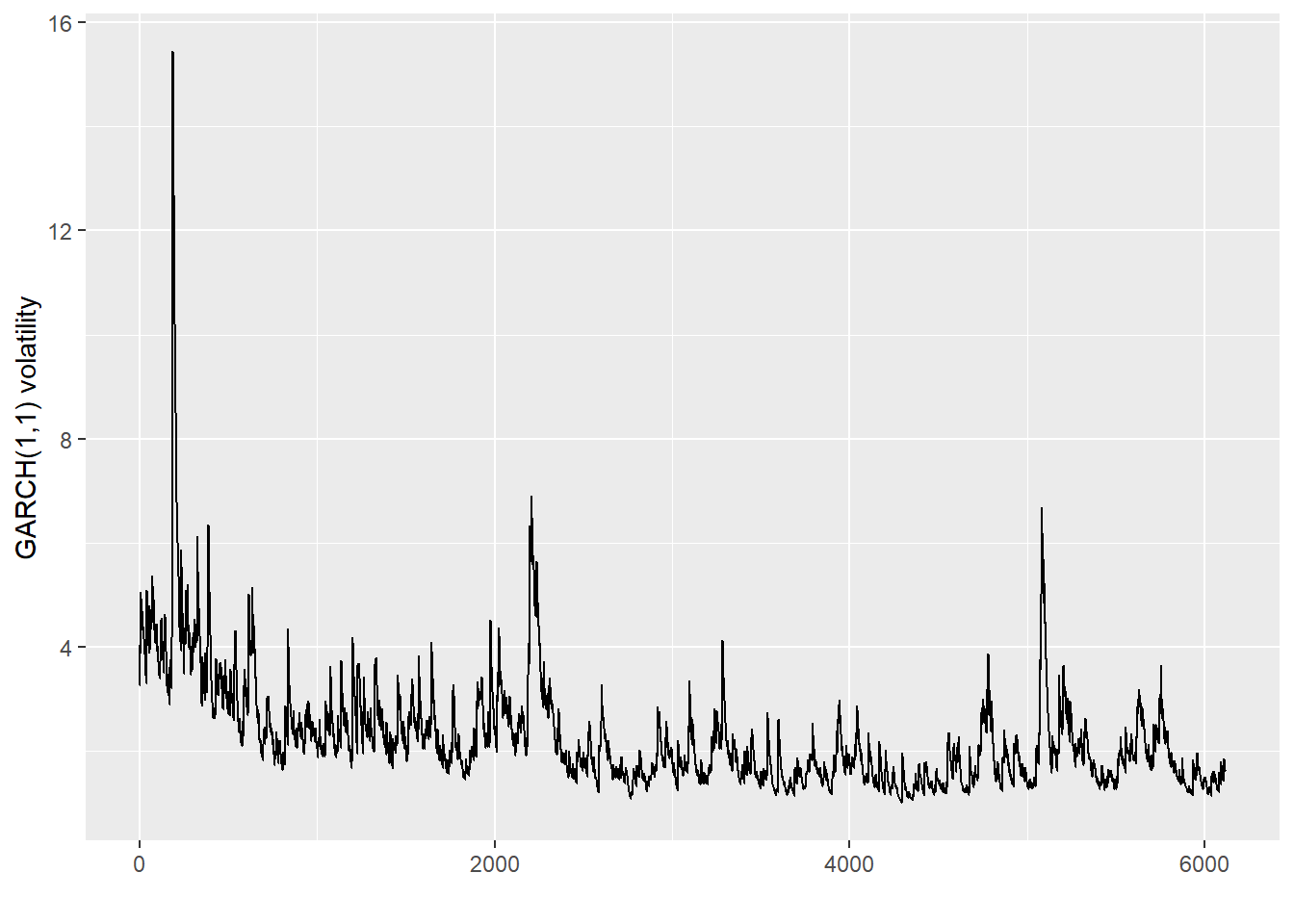
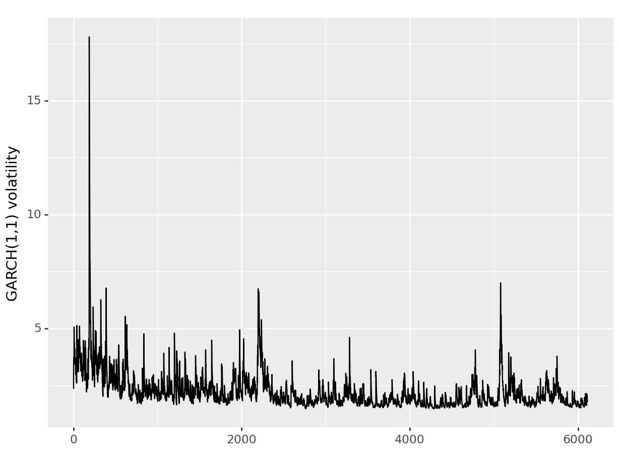
Next, I plot the time series of the estimated conditional variances \(\sigma_t\) based on the output. To keep the required code clean and simple, my function logL_garch returns the fitted variances with the option return_only_loglik = FALSE.

R
Python

tibble(vola = logL_garch(fitted_garch_params, p, q, ret, FALSE)) |> 
  ggplot(aes(x = 1:length(vola), y = sqrt(vola))) +
  geom_line() +
  labs(x = "", y  = "GARCH(1,1) volatility")

# Assuming you have the 'fitted_garch_params' and 'ret' variables already defined
vola = logL_garch(fitted_garch_params, p, q, ret, return_only_loglik=False)

# Create a pandas DataFrame
df = pd.DataFrame({'vola': vola})

# Plotting
(ggplot(df, aes(x=df.index + 1, y=df['vola'].apply(np.sqrt))) +
 geom_line() +
 labs(x='', y='GARCH(1,1) volatility'))

<Figure Size: (640 x 480)>

Next, the typical tidyverse approach: Once we implement the workflow for one asset, we can use mutate and map() to perform the exact computation in a tidy manner for all assets in our sample. The lecture slides define the unconditional variance.

R
Python

unconditional_volatility <- returns |> 
  arrange(symbol, date) |> 
  nest(data = c(date, ret)) |> 
  mutate(arch = map(data, function(.x){
    
    ret <- .x |> pull(ret) 
    p <- 2
    initial_params <- (c(sd(ret), rep(1, p)))
    fit_manual <- optim(par = initial_params, 
                        fn = logL_arch, 
                        hessian = TRUE, 
                        method="L-BFGS-B", 
                        lower = 0, 
                        p = p,
                        ret = ret)
    
    fitted_params <- (fit_manual$par)
    se <- sqrt(diag(solve(fit_manual$hessian)))
    
    return(tibble(param = c("intercept", paste0("alpha_", 1:p)),
                  value = fitted_params, se = se))
  })) |> 
  select(-data) |> 
  unnest(arch) |>
  summarise(uncond_var = dplyr::first(value) / (1 - sum(value) + dplyr::first(value)))
  
unconditional_volatility |> 
  ggplot() + 
  geom_bar(aes(x = reorder(symbol, uncond_var), 
               y = sqrt(250) * uncond_var), stat = "identity") + 
  coord_flip() +
  labs(x = "Unconditional volatility (annualized)", 
      y = "")

# Arrange the DataFrame by 'symbol' and 'date'
returns = returns.sort_values(by=['symbol', 'date'])

# Group by 'symbol' and nest 'date' and 'ret' columns
nested_data = returns.groupby('symbol')[['date', 'ret']].apply(lambda x: x.values.tolist())

# Calculate ARCH model parameters and unconditional volatility for each symbol
results = []
for data in nested_data:
    ret = np.array([x[1] for x in data])
    p = 2
    initial_params = np.concatenate(([np.std(ret)], np.ones(p)))
    fit_manual = minimize(logL_arch, initial_params, args=(p, ret), method='L-BFGS-B', bounds=[(0, None)] * (p + 1))
    fitted_params = fit_manual.x
    uncond_var = fitted_params[0] / (1 - np.sum(fitted_params[1:]) + fitted_params[0])
    results.append(uncond_var)

# Create DataFrame of unconditional volatility for each symbol
unconditional_volatility = pd.DataFrame({'symbol': nested_data.index, 'uncond_var': results})

# Plotting
#(
#    ggplot(unconditional_volatility) +
#    geom_bar(aes(x='symbol', y='sqrt(250) * uncond_var'), stat="identity") +
#    coord_flip() +
#    labs(x="Unconditional volatility (annualized)", y="")
#)

For an illustration of the value at risk computation, consult the lecture slides.

Ledoit-Wolf shrinkage estimation

A severe practical issue with the sample variance-covariance matrix in large dimensions (\(N >>T\)) is that \(\hat\Sigma\) is singular. Ledoit and Wolf proposed a series of biased estimators of the variance-covariance matrix \(\Sigma\), which overcome this problem. As a result, it is often advised to perform Ledoit-Wolf-like shrinkage on the variance-covariance matrix before proceeding with portfolio optimization.

Exercises:

Read the introduction of the paper Honey, I shrunk the sample covariance matrix and implement the feasible linear shrinkage estimator. If in doubt, consult Michael Wolf’s homepage. You will find helpful R and Python codes there.
Write a simulation that generates iid distributed returns (you can use the random number generator rnorm()) for some dimensions \(T \times N\) and compute the minimum-variance portfolio weights based on the sample variance-covariance matrix and Ledoit-Wolf shrinkage. What is the mean squared deviation from the optimal portfolio (\(1/N\))? What can you conclude?

Solutions:

The assignment requires you to understand the original paper in depth - it is arguably hard to translate the derivations into working code. However, below are some sample codes you can use for future assignments.

compute_ledoit_wolf <- function(x) {
  # Computes Ledoit-Wolf shrinkage covariance estimator
  # This function generates the Ledoit-Wolf covariance estimator  as proposed in Ledoit, Wolf 2004 (Honey, I shrunk the sample covariance matrix.)
  # X is a (t x n) matrix of returns
  t <- nrow(x)
  n <- ncol(x)
  x <- apply(x, 2, function(x) if (is.numeric(x)) # demean x
    x - mean(x) else x)
  sample <- (1/t) * (t(x) %*% x)
  var <- diag(sample)
  sqrtvar <- sqrt(var)
  rBar <- (sum(sum(sample/(sqrtvar %*% t(sqrtvar)))) - n)/(n * (n - 1))
  prior <- rBar * sqrtvar %*% t(sqrtvar)
  diag(prior) <- var
  y <- x^2
  phiMat <- t(y) %*% y/t - 2 * (t(x) %*% x) * sample/t + sample^2
  phi <- sum(phiMat)

  repmat = function(X, m, n) {
    X <- as.matrix(X)
    mx = dim(X)[1]
    nx = dim(X)[2]
    matrix(t(matrix(X, mx, nx * n)), mx * m, nx * n, byrow = T)
  }

  term1 <- (t(x^3) %*% x)/t
  help <- t(x) %*% x/t
  helpDiag <- diag(help)
  term2 <- repmat(helpDiag, 1, n) * sample
  term3 <- help * repmat(var, 1, n)
  term4 <- repmat(var, 1, n) * sample
  thetaMat <- term1 - term2 - term3 + term4
  diag(thetaMat) <- 0
  rho <- sum(diag(phiMat)) + rBar * sum(sum(((1/sqrtvar) %*% t(sqrtvar)) * thetaMat))

  gamma <- sum(diag(t(sample - prior) %*% (sample - prior)))
  kappa <- (phi - rho)/gamma
  shrinkage <- max(0, min(1, kappa/t))
  if (is.nan(shrinkage))
    shrinkage <- 1
  sigma <- shrinkage * prior + (1 - shrinkage) * sample
  return(sigma)
}

The simulation can be conducted as below. First, the individual functions simulate iid normal “returns” matrix for given dimensions T and N. Next, optimal weights are computed using either the variance-covariance matrix or the Ledoit-Wolf shrinkage equivalent. If you want to generate results that can be replicated, use the function set.seed(). It takes any integer as input and ensures that whoever runs this code afterward retrieves the same random numbers within the simulation. Otherwise (or if you change “2023” to an arbitrary other value), there will be some variation in the results because of the random sampling of returns.

set.seed(2023)

generate_returns <- function(T, N) matrix(rnorm(T * N), nc = N)

# Minimum variance portfolio weights
compute_mvp_sample <- function(mat){
  w <- solve(cov(mat))%*% rep(1,ncol(mat))
  return(w/sum(w))
}
compute_mvp_lw <- function(mat){
  w <- solve(compute_ledoit_wolf(mat))%*% rep(1,ncol(mat))
  return(w/sum(w))
}

eval_weight <- function(w) length(w)^2 * sum((w - 1/length(w))^2)

Note that I evaluate weights based on the squared deviations from the naive portfolio (the minimum variance portfolio in the case of iid returns). The scaling length(w)^2 is just there to penalize larger dimensions harder.

simulation <- function(T = 100, N = 70){
  simulation_rounds <- 50 
  tmp <- matrix(NA, nc = 2, nr = simulation_rounds)
  for(i in 1:simulation_rounds){
    mat <- generate_returns(T, N)
    w_lw <- compute_mvp_lw(mat)
    if(N < T) w_sample <- compute_mvp_sample(mat)
    if(N >= T) w_sample <- rep(NA, N)
    tmp[i, 1] <- eval_weight(w_lw)
    tmp[i, 2] <- eval_weight(w_sample)
  }
  tibble(model = c("Shrinkage", "Sample"), error = colMeans(tmp), N = N, T = T)
}

result <- bind_rows(simulation(100, 60),
                    simulation(100, 70),
                    simulation(100, 80),
                    simulation(100, 90),
                    simulation(100, 100),
                    simulation(100, 150))

result |> 
  pivot_wider(names_from = model, values_from = error) |>
  knitr::kable(digits = 2, "pipe")

N	T	Shrinkage	Sample
60	100	1.30	89.59
70	100	1.51	164.15
80	100	1.60	305.91
90	100	1.99	874.19
100	100	2.23	NA
150	100	3.29	NA

The results show a couple of interesting results: First, the sample variance-covariance matrix breaks down if \(N > T\) - no unique minimum variance portfolio anymore. On the contrary, Ledoit-Wolf-like shrinkage retains the positive definiteness of the estimator even if \(N > T\). Further, the (scaled) mean-squared error of the portfolio weights relative to the theoretically optimal naive portfolio is way smaller for the Shrinkage version. Although the variance-covariance estimator is biased, the variance of the estimator is reduced substantially and thus provides more robust portfolio weights.