In these exercises, you familiarize yourself with the details behind shrinkage regression methods such as Ridge and Lasso. Although R and Python provide amazing interfaces which perform the estimation flawlessly, you are first asked to implement Ridge and Lasso regression estimators from scratch before moving on to using the package glmnet next.
Introduction to penalized regressions
Exercises:
Load the file macro_predictors from the tidy_finance_*.sqlitedatabase. Create a variable ythat contains the market excess returns from the Goyal-Welsh dataset (rp_div) and a matrix X that contains the remaining macroeconomic variables except for the column month. You will use X and y to perform penalized regressions. Try to run a simple linear regression of X on `y´ to analyze the relationship between the macroeconomic variables and market returns. Which problems do you encounter?
Write a function that requires three inputs, y (a \(T\) vector), X (a \((T \times K)\) matrix), and lambda and which returns the Ridge estimator (a \(K\) vector) for given penalization parameter \(\lambda\). Recall that the intercept should not be penalized. Therefore, your function should allow you to indicate whether \(X\) contains a vector of ones as the first column which should be exempt from the \(L_2\) penalty.
Compute the \(L_2\) norm (\(\beta'\beta\)) for the regression coefficients based on the predictive regression from the previous exercise for a range of \(\lambda\)’s and illustrate the effect of the penalization in a suitable figure.
Now, write a function that requires three inputs, y (a \(T\) vector), X (a \((T \times K)\) matrix), and ’lambda` and which returns the Lasso estimator (a \(K\) vector) for given penalization parameter \(\lambda\). Recall that the intercept should not be penalized. Therefore, your function should allow you to indicate whether \(X\) contains a vector of ones as the first column which should be exempt from the \(L_1\) penalty.
After you are sure you understand what Ridge and Lasso regression are doing, familiarize yourself with the documentation of the package glmnet(). It is a thoroughly tested and well-established package that provides efficient code to compute the penalized regression coefficients not only for Ridge and Lasso but also for combinations, therefore, commonly called elastic nets.
── Attaching core tidyverse packages ──────────────────────── tidyverse 2.0.0 ──
✔ dplyr     1.1.4     ✔ readr     2.1.4
✔ forcats   1.0.0     ✔ stringr   1.5.1
✔ ggplot2   3.4.4     ✔ tibble    3.2.1
✔ lubridate 1.9.3     ✔ tidyr     1.3.0
✔ purrr     1.0.2
── Conflicts ────────────────────────────────────────── tidyverse_conflicts() ──
✖ dplyr::filter() masks stats::filter()
✖ dplyr::lag()    masks stats::lag()
ℹ Use the conflicted package (<http://conflicted.r-lib.org/>) to force all conflicts to become errors
# Read in the datatidy_finance <-dbConnect(SQLite(),"../AEF_2024/data/tidy_finance_r.sqlite",extended_types =TRUE)macro_predictors <-tbl(tidy_finance, "macro_predictors") |>collect()y <- macro_predictors$rp_divX <- macro_predictors |>select(-month, -rp_div) |>as.matrix()# OLS for Welsh data fails because X is not of full rankc(ncol(X), Matrix::rankMatrix(X))
[1] 13 11
import pandas as pdimport requestsimport numpy as npfrom io import BytesIO, StringIOimport zipfileimport sqlite3from plotnine import ggplot, aes, geom_line, labsfrom scipy.optimize import minimize#Read the datatidy_finance = sqlite3.connect(database="../AEF_2024/data/tidy_finance_python.sqlite")macro_predictors = pd.read_sql_query( sql="SELECT * FROM macro_predictors", con=tidy_finance)y = macro_predictors['dp'].valuesX = macro_predictors.drop(columns=['month', 'dp']).values# OLS for Welsh data fails because X is not of full rankprint(X.shape[1], np.linalg.matrix_rank(X))
12 11
As for OLS, the objective function is to minimize the sum of squared errors \((y - X\beta)'(y - X\beta)\) under the condition that \(\sum\limits_{j=2}^K \beta_j \leq t(\lambda)\)if an intercept is present. This can be rewritten as \(\beta'A\beta \leq t(\lambda)\) where \(A = \begin{pmatrix}0&&\ldots&&0\\\vdots& 1&0&\ldots&0\\&\vdots&\ddots&&0\\0& &\ldots&&1\end{pmatrix}\). Otherwise, the condition is simply that \(\beta'I_K\beta \leq t(\lambda)\) where \(I_k\) is an identity matrix of size (\(k \times k\)).
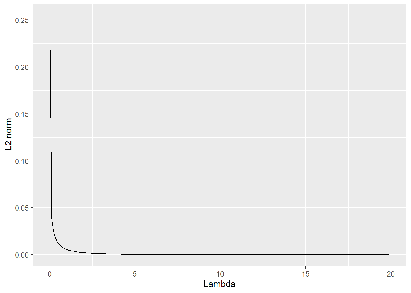
Finally, the following code sequence computes the \(L_2\) norm of the ridge regression coefficients for a given \(\lambda\). Note that to implement this evaluation in a tidy manner, vectorized functions are important! R provides great ways to vectorize a function, to learn more, Hadley Wickham’s book Advanced R is a highly recommended read!
l2_norm <-function(lambda) sum(ridge_regression(y = y, X = X, lambda = lambda)^2) # small helper function to extract the L_2 norm of the ridge regression coefficientsl2_norm <-Vectorize(l2_norm) # To use the function within a `mutate` operation, it needs to be vectorizedseq(from =0.01, to =20, by =0.1) |>as_tibble() |>mutate(norm =l2_norm(value)) |>ggplot(aes(x = value, y = norm)) +geom_line() +labs(x ="Lambda", y =" L2 norm")
To compute the coefficients of linear regression with a penalty on the sum of the absolute value of the regression coefficients, numerical optimization routines are required. Recall, the objective function is to minimize the sum of squared residuals, \(\hat\varepsilon'\hat\varepsilon\) under the constraint that \(\sum\limits_{j=2}^K\beta_j\leq t(\lambda)\). Make sure you familiarize yourself with the way, numerical optimization in R works: we first define the objective function (objective_lasso()) which has the parameter we aim to optimize as its first argument. The main function lasso_regression() then only calls this helper function.
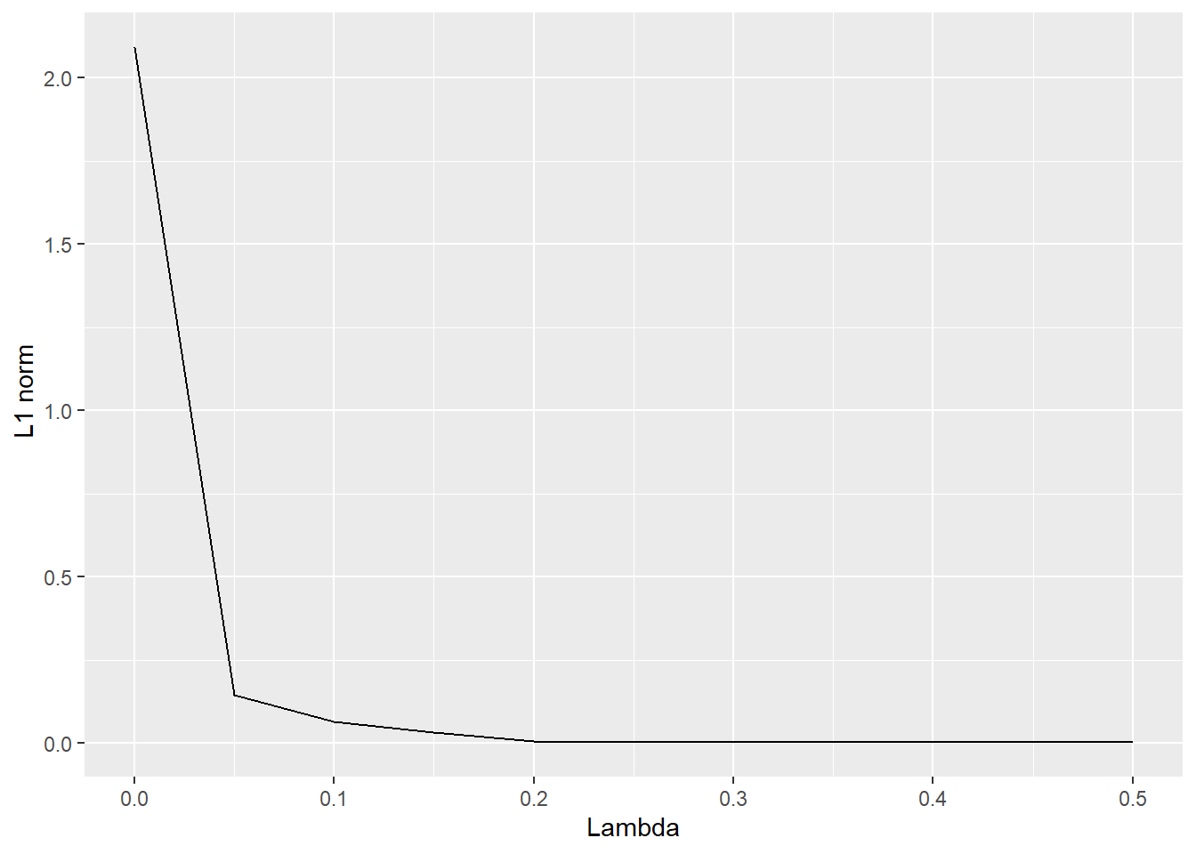
Finally, as in the previous example with Ridge regression, I illustrate how a larger penalization term \(\lambda\) affects the \(L_1\) norm of the regression coefficients.
l1_norm <-function(lambda) sum(abs(lasso_regression(y = y, X = X, lambda = lambda)))l1_norm <-Vectorize(l1_norm) # To use the function within a `mutate` operation, it needs to be vectorizedseq(from =0, to =0.5, by =0.05) |>as_tibble() |>mutate(norm =l1_norm(value)) |>ggplot(aes(x = value, y = norm)) +geom_line() +labs(x ="Lambda", y =" L1 norm")
While the code above should work, there are well-tested R packages available that provide a much more reliable and faster implementation. Thus, you can safely use the package glmnet. As a first step, the following code create the sequence of regressions coefficients for the Goyal-Welch dataset which should be identical to the example we discussed in the lecture slides.
Note the function argument alpha. glmnet() allows a more flexible combination of \(L_1\) and \(L_2\) penalization on the regression coefficients. The pure ridge estimation is implemented with alpha = 0, lasso requires alpha = 1.
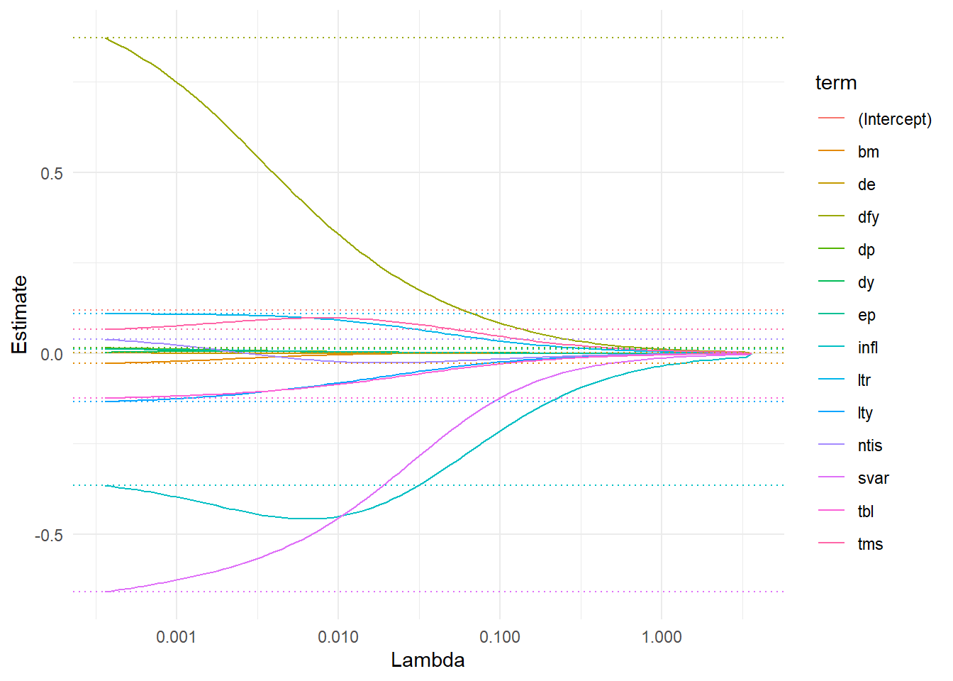
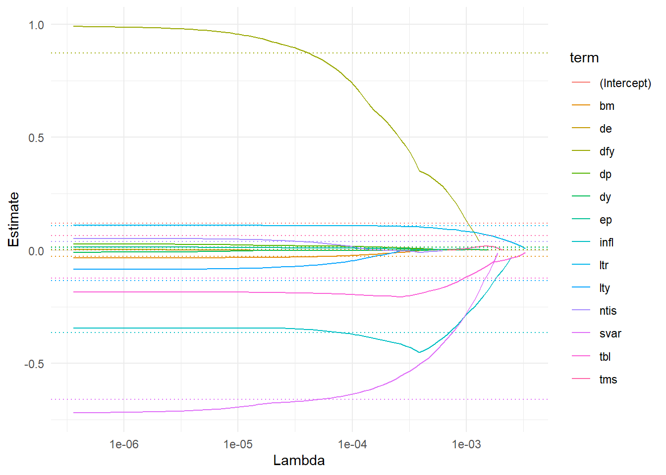
fit_lasso <-glmnet(X, y, # Modelalpha =1)broom::tidy(fit_lasso) |>filter(term !="(Intercept)") |>ggplot(aes(x = lambda, y = estimate, color = term)) +geom_line() +geom_hline(data = broom::tidy(fit_ridge) |>filter(lambda ==min(lambda)),aes(yintercept = estimate, color = term), linetype ="dotted") +theme_minimal() +scale_x_log10() +labs(x ="Lambda", y ="Estimate")
# import glmnet# # Lasso and Ridge regression# fit_lasso = glmnet.elnet(X, y, alpha=1)# # # Using broom to tidy up the results# tidy_results = pd.DataFrame({# 'term': fit_lasso.get_vnames()[1:],# 'lambda': fit_lasso.lambda_,# 'estimate': fit_lasso.coef_[1:]# })# # # Filtering out the intercept term# tidy_results = tidy_results[tidy_results['term'] != "(Intercept)"]# # # Plotting# (ggplot(tidy_results, aes(x='lambda', y='estimate', color='term')) +# geom_line() +# geom_hline(data=tidy_results[tidy_results['lambda'] == min(tidy_results['lambda'])],# aes(yintercept='estimate', color='term'), linetype='dotted') +# theme_minimal() +# scale_x_log10() +# labs(x='Lambda', y='Estimate'))
Note in the figure how Lasso discards all variables for high values of \(\lambda\) and then gradually incorporates more predictors. It seems like stock variance is selected first. As expected, for \(\lambda \rightarrow 0\), the lasso coefficients converge towards the OLS estimates (illustrated with dotted lines).
Factor selection via machine learning
In this Chapter, you get to know tidymodels (R) and scikit-learn (Python), a collection of packages for modeling and machine learning (ML) using tidy coding principles. From a finance perspective, you will apply penalized regressions to understand which factors and macroeconomic predictors may help to explain the cross-section of industry returns.
Exercises:
In this analysis, we use four different data sources. Load the monthly Fama-French 3-factor returns, the monthly q-factor returns from Hou, Xue, and Zhang (2014), the macroeconomic predictors from Welch and Goyal (2008), and monthly portfolio returns from 10 different industries according to the definition from Kenneth French’s homepage as test assets. Your data should contain 22 columns of regressors with 13 macro variables and 8-factor returns for each month.
Provide meaningful summary statistics for the test assets’ excess returns.
Familiarize yourself with the tidymodels workflow. First, restrict yourself to just one industry, e.g. Manufacturing. Use the function initial_time_split from the rsample package to split the sample into a training and a test set.
Preprocess the data by creating a recipe which performs the following steps: First, the aim is to explain the industry excess returns as a function of all predictors. Exclude the column month from the analysis. Include all interaction terms between factors and macroeconomic predictors. Demean and scale each regressor such that the standard deviation is one.
Build a model linear_reg with tidymodels with a fixed penalty term that performs lasso regression. Create a workflow that first applies the recipe steps to the training data and then fits the model. Illustrate the predicted industry returns for the in-sample and the out-of-sample period.
Next, tune the model such that the penalty term is flexibly chosen by cross-validation. For that purpose, update the model such that both, penalty and mixture are flexible tuning variables. Use the function time_series_cv to generate a time series cross-validation sample which allows tuning the model with 20 random samples of length five years with a validation period of four years. Tune the model for a grid of possible penalty and mixture values and visualize the mean-squared prediction errors for the industry returns across the range of possible tuning parameters.
Finally, write a function to parallelize the entire workflow. The function should split the data into a training and test set, create a cross-validation scheme, and tunes a lasso model for different penalty values. Finally, select the best model in terms of MSPE in the validation test set. Apply the function to every individual industry and illustrate for each industry which factor and macroeconomic variables are selected by the Lasso.
Familiarize yourself with the scikit-learn workflow. First, restrict yourself to just one industry, e.g. Manufacturing. Use the function train_test_split to split the sample into a training and a test set.
Preprocess the data with ColumnTransformer which performs the following steps: First, the aim is to explain the industry excess returns as a function of all predictors. Exclude the column month from the analysis. Include all interaction terms between factors and macroeconomic predictors. Demean and scale each regressor such that the standard deviation is one.
Build a model ElasticNet with sklearn.linear_model with a fixed penalty term that performs lasso regression. Create a Pipeline that first applies the recipe steps to the training data and then fits the model. Illustrate the predicted industry returns for the in-sample and the out-of-sample period.
Next, tune the model such that the penalty term is flexibly chosen by cross-validation. For that purpose, update the model such that both, penalty and mixture are flexible tuning variables. Use the function TimeSeriesSplit to generate a time series cross-validation sample which allows tuning the model with 20 random samples of length five years with a validation period of four years. Tune the model for a grid of possible penalty and mixture values and visualize the mean-squared prediction errors for the industry returns across the range of possible tuning parameters.
Finally, write a function to parallelize the entire workflow. The function should split the data into a training and test set, create a cross-validation scheme, and tunes a lasso model for different penalty values. Finally, select the best model in terms of MSPE in the validation test set. Apply the function to every individual industry and illustrate for each industry which factor and macroeconomic variables are selected by the Lasso.
Solutions: All solutions are provided in the book chapter Factor selection via machine learning (R or Python version).